Continual learning research · earlier models, 2025 – October 2026
The AI players built so far, head to head
The models built before the gated test and how they fared against each other in the combat arena.
The proposed research loop
One agent. Many games. Learning to change its own code.
Carry learned weights across environments, keep learning through interaction, and learn which edits to the model’s own code improve its future learning.
Proposed design · Not implemented in Lana · Transfer, retention and useful self-editing remain unproven.
Train in a game
Observe → act → task reward → update model weights.
Direct a model-code edit
At a checkpoint, an editing controller chooses an instruction for an external code editor, or skips editing.
Train and evaluate the candidate
Test the revised model against a matched unchanged learner; check performance and retention across games.
Learn which edits help
Use measured improvement, forgetting and compute cost as reward to update the editing controller. Keep or revert the patch.
Switch games, carry weights
Swap the environment and observation/action adapter. Continue from the current learned weights.
Revisit earlier games
Evaluate the latest weights to measure retained skills. Feed development results into the next cycle.
Repeat ordinary RL updates within each game; code edits and game switches happen at declared checkpoints, not after every action. Preserve compatible weights through code changes and explicitly initialize any new parameters. Returning to an earlier game uses the latest weights, not its old checkpoint.
The external editor writes candidate patches; the learned controller decides when and how to request them. This design works without access to the editor’s weights. The runner independently trains, evaluates and accepts or rejects each candidate.
Games and their adapters come from a defined schedule. The agent learns to edit its model; this proposal does not ask it to design games. Edit rewards use development evaluations, while the final evaluation suite stays separate.
Inside the combat agent
MuZero: learn to predict, search to act.
Our independent MuZero implementation, shown with the J checkpoint’s settings. Past observations become a compact state; learned predictions guide a search for actions that lead to winning.
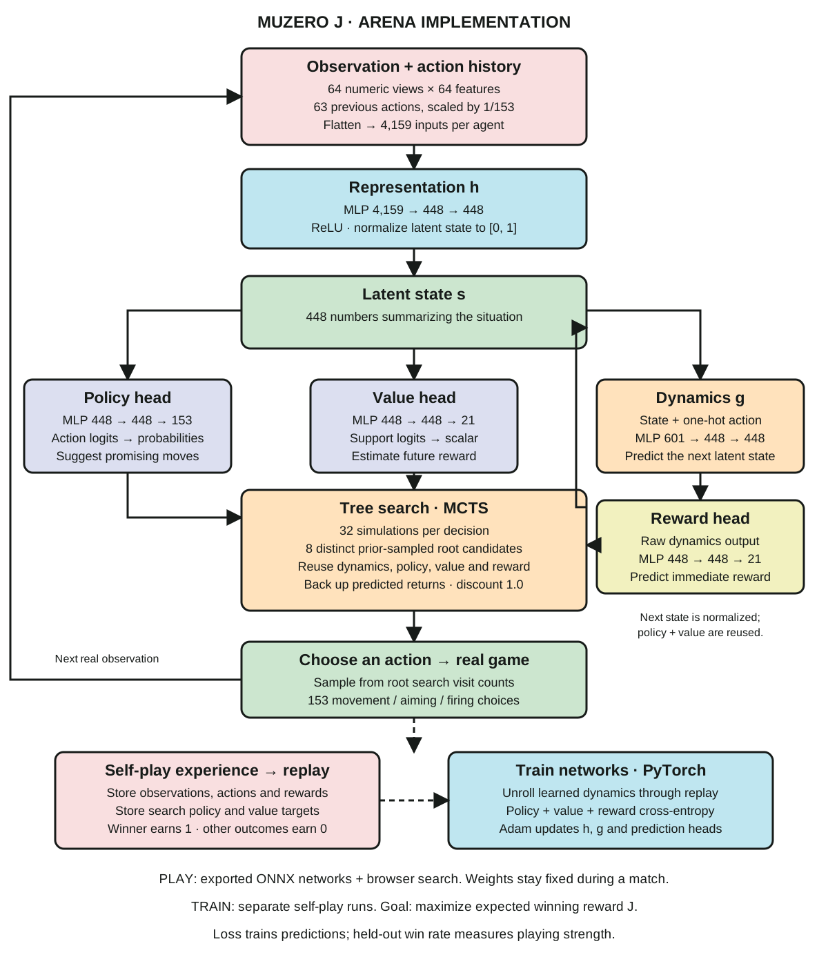
How each part works · implementation details
- History, not a Transformer
- Each agent gets its own window of 64 numeric observations and 63 previous actions. Missing early history is zero-padded. The flattened vector feeds a two-layer MLP.
- Learned world model
- Dynamics predict a latent next state, not pixels or the full game board. The reward head reads the raw dynamics output; policy and value read the normalized state. Search never calls the real game simulator.
- Policy, value and reward
- All heads use Linear → ReLU → Linear. Policy has 153 action logits. Value and reward use 21 support bins, decoded with the inverse scalar transform; they are not direct probability outputs.
- Planning
- J uses 32 search simulations, 8 distinct prior-sampled root candidates and discount 1.0. Learned policy priors guide exploration; predicted rewards and leaf values are backed up. These settings differ from older combat checkpoints.
- Learning to win
- Self-play creates replay data and search-policy targets. Training minimizes policy, value and reward prediction losses over unrolled sequences. The objective is expected winning reward; evaluation win rate determines whether play improved.
- Playing is not training
- The site runs exported networks with browser search. It does not update weights during your match. This diagram describes an experimental implementation, not evidence of superhuman performance.
Self-play and training source · Batched search source · Download diagram (SVG)
Inside the research model
Observe. Imagine. Plan. Learn.
Each box shows its structure, how it helps the model and a loose brain analogy. The comparisons describe similar roles, not biological equivalence.
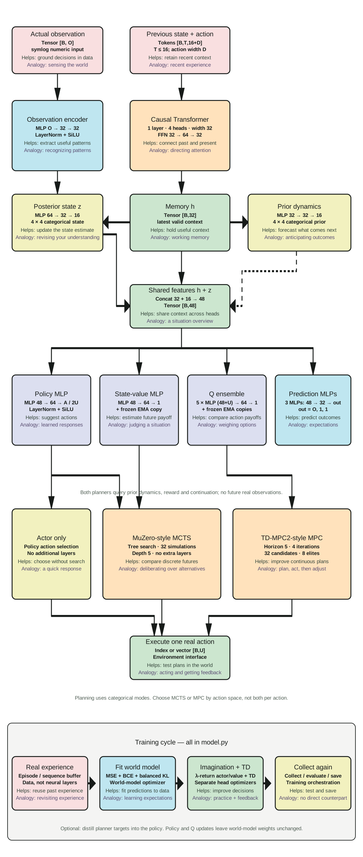
Complete network · default configuration
B = batch size; O = observation width; A = discrete action count; U = continuous action width; D = A or U. Dimensions are configurable. This map describes HybridModel in model.py at 4b54ed9.
W(in, out) = Linear(in, 32) → LayerNorm(32) → SiLU → Linear(32, out). H(in, out) = Linear(in, 64) → LayerNorm(64) → SiLU → Linear(64, out). All Linear layers include bias. Algorithm and data boxes add no neural layers.
- Actual observation
- Input x: [B, O]; apply symlog before encoding.
- Previous state + action
- Concatenate flatten(z): 16 with previous action: D. Tokens [B, T, 16+D], T ≤ 16. D=A one-hot for discrete actions, D=U normalized coordinates for continuous actions.
- Observation encoder
- W(O, 32): Linear O→32 → LayerNorm(32) → SiLU → Linear 32→32. Encoded observation e: [B, 32].
- Causal Transformer
- Linear (16+D)→32 + learned positions [1,16,32]. One pre-norm block: LN → 4-head causal self-attention (8 dimensions/head; QKV 32→96, output 32→32) → residual; LN → Linear 32→64 → GELU → Linear 64→32 → residual. Final LayerNorm(32). Dropout 0; causal and padding masks.
- Posterior state z
- Concatenate h and e: [B,64] → W(64,16) → reshape [B,4,4]. Four categorical variables, four classes each; 0.01 uniform probability mix. Straight-through one-hot samples during learning; categorical modes in planning.
- Memory h
- Latest valid Transformer output h: [B,32]. Rolling per-stream token buffer; no additional recurrent layer.
- Prior dynamics
- h: [B,32] → W(32,16) → categorical logits [B,4,4], same uniform mix as posterior. Next h comes from Transformer(previous z, action); prior predicts next z without an actual observation.
- Shared features h + z
- Concatenate h: [B,32] and flatten(z): [B,16] → features f: [B,48]. No trainable layer.
- Policy MLP
- Discrete: H(48,A) → logits [B,A] → Categorical. Continuous: H(48,2U) → mean μ and scale s; σ=0.1+0.9·sigmoid(s); tanh(Normal(μ,σ)) actions [B,U]. Mean action is tanh(μ).
- State-value MLP
- H(48,1) → scalar V [B,1] in raw reward units. Frozen target copy updated by EMA (default 0.99).
- Q ensemble
- Continuous actions only: five independent H(48+U,1) critics on concat(f,action), stacked output [5,B]. Five frozen EMA target copies. Real TD target uses minimum of two sampled target critics; MPC horizon uses mean of two sampled critics.
- Prediction MLPs
- Three independent world heads: decoder W(48,O), reward W(48,1), continuation W(48,1). Outputs [B,O], [B,1], [B,1]. Decoder/reward predict symlog values; continuation is a logit → sigmoid. Reward uses symexp for planning returns.
- Actor only
- Action selection algorithm, no extra neural layers. Samples or selects from the policy output.
- MuZero-style MCTS
- Tree-search algorithm, no extra neural layers. Defaults: 32 simulations, horizon 5. Uses actor priors, prior latent transitions, reward/continuation and state-value leaves; selects from root visit counts.
- TD-MPC2-style MPC
- Action-sequence optimization, no extra neural layers. Defaults: horizon 5, 32 candidates, 4 actor candidates, 8 elites, 4 iterations. Weighted elites and shifted warm start; Q terminal score (state-value ablation available).
- Execute one real action
- Environment interface: discrete index [B] or continuous bounded vector [B,U]. Execute one action, then ingest the next real observation.
- Real experience / replay
- Episode/sequence replay data structure storing real observations, actions, rewards and termination/truncation boundaries; no neural layers.
- Fit world model
- World-model optimizer: symlog reconstruction/reward MSE, continuation BCE, balanced categorical KL with free nats (1). Default KL scales: dynamics 1, representation 0.1.
- Imagination + TD
- Frozen-world imagination (default horizon 5): score-function actor, λ-return value learning (λ=.95, γ=.99), slow-value regularization. Continuous critics: real replay TD with actual next posterior. Separate head updates; no world gradients.
- Collect again / checkpoint
- Collection/evaluation/checkpoint orchestration, no neural layers. Saves model, optimizer and training state for continuation.
- Optional planner distillation
- Optional loss on the existing actor, no new layers: categorical cross-entropy or continuous mean MSE against planner targets. Weight 0 by default.
Every part: how it helps and the brain analogy
- Actual observation
- Helps the model: Supplies the current numeric view so decisions can respond to what is happening.
- Brain analogy: Like receiving sensory information; these inputs are numeric vectors, not biological senses.
- Previous state + action
- Helps the model: Carries earlier latent states and actions forward so the model can use temporal context.
- Brain analogy: Like keeping track of what just happened and what you just did.
- Observation encoder
- Helps the model: Transforms numeric observations into features that help infer the current state.
- Brain analogy: Like extracting useful patterns from sensory input; it is not a model of sensory cortex.
- Causal Transformer
- Helps the model: Weights and combines past state/action tokens; causal masking prevents access to future tokens.
- Brain analogy: Like attending to relevant context. Transformer attention is a mathematical operation, not biological attention.
- Posterior state z
- Helps the model: Combines current evidence with memory to infer a compact categorical state.
- Brain analogy: Like revising your understanding when you see new evidence; categorical variables are an engineering choice.
- Memory h
- Helps the model: Provides a context vector from the recent history window to the other components.
- Brain analogy: Like temporarily holding task-relevant information in working memory; this is not proven long-term skill retention.
- Prior dynamics
- Helps the model: Predicts categorical states during imagination and search, without future real observations.
- Brain analogy: Like anticipating a possible outcome before it happens; this is not evidence of conscious imagination.
- Shared features h + z
- Helps the model: Joins memory and latent state so the policy and prediction heads use a common representation.
- Brain analogy: Like combining recent context with your current interpretation; no single brain location is implied.
- Policy MLP
- Helps the model: Produces discrete action probabilities or a continuous action distribution; it also proposes actions to search.
- Brain analogy: Like a learned action tendency. Fast policy output is not proof of a human habit mechanism.
- State-value MLP
- Helps the model: Estimates expected discounted reward from a state when following the actor.
- Brain analogy: Like judging whether a situation is promising, not a feeling or a conscious judgment.
- Q ensemble
- Helps the model: Scores a state and continuous action with several critics; target estimates train from real replay and Q values guide MPC.
- Brain analogy: Like comparing possible payoffs. The ensemble itself has no claimed biological counterpart.
- Prediction MLPs
- Helps the model: Reconstruction helps train representations; reward and continuation predictions score imagined futures.
- Brain analogy: Like having expectations about outcomes. A reward number is not pleasure, and continuation is not self-awareness.
- Actor only
- Helps the model: Uses the policy directly when planning is disabled, avoiding planner computation.
- Brain analogy: Like responding quickly from a learned tendency rather than mentally comparing several futures.
- MuZero-style MCTS
- Helps the model: Uses policy priors, cached latent transitions and state-value estimates to explore discrete alternatives.
- Brain analogy: Like deliberating over alternatives. This implementation does not claim the brain runs this MCTS algorithm.
- TD-MPC2-style MPC
- Helps the model: Optimizes bounded action sequences, executes one action, and replans after the next actual observation.
- Brain analogy: Like planning a movement and correcting it with new feedback; it does not reproduce biological motor circuits.
- Execute one real action
- Helps the model: Applies a selected action in the environment so the next observation can confirm or contradict predictions.
- Brain analogy: Like acting and receiving new feedback; execution is performed by the environment interface.
- Real experience / replay
- Helps the model: Stores complete episodes for repeated learning rather than discarding each transition after one update.
- Brain analogy: Loosely resembles memory reactivation. A software replay buffer does not model sleep or hippocampal circuitry.
- Fit world model
- Helps the model: Uses reconstruction, reward, continuation and prior/posterior losses to improve the learned world model.
- Brain analogy: Like adjusting expectations after experience; backpropagation here is not a claimed biological learning mechanism.
- Imagination + TD
- Helps the model: Learns policy/value from predicted trajectories and continuous Q values from real rewards and actual next observations.
- Brain analogy: Like mental rehearsal and learning when outcomes differ from expectations; these are functional analogies.
- Collect again / checkpoint
- Helps the model: Collects fresh episodes, evaluates behavior and saves training state for reproducible continuation.
- Brain analogy: Evaluation and disk checkpoints are engineering tools, not brain structures or memory consolidation.
- Optional planner distillation
- Helps the model: Trains the policy to imitate recent planner choices, reducing reliance on search when imitation is useful. It is off by default.
- Brain analogy: Like practicing a considered decision until a quicker response is possible; this does not establish habit learning or lasting skill retention.
Working memory involves holding and updating useful information temporarily (NIMH). Human hippocampal replay has been linked to later memory performance (Schapiro et al., 2018). These motivate comparisons; they do not validate this model as a brain simulation.
Implementation and limits
- Transformer memory
- Causal attention over recent numeric states and actions. Each stream has its own history; observations are not text.
- Dreamer-style world model
- Actual observations infer a categorical posterior. Prior dynamics imagine future states and predict reward and continuation. The decoder is used for training, not required by search.
- MuZero-style MCTS
- For discrete actions, search uses policy priors, cached latent transitions, state-value leaves and discounted backups. Root visits select an action; observed legality applies at the root.
- TD-MPC2-style MPC
- For continuous actions, optimize bounded action sequences with actor proposals, weighted elites and a shifted warm start. A separate Q ensemble supplies the horizon value; state value is an optional ablation.
- Imagination, TD & distillation
- Train policy and state value on imagined returns, and continuous Q critics on real replay. Planner distillation is optional and off by default. These updates do not change world-model weights.
- One model file, full training loop
- model.py contains the networks, MCTS/MPC, replay, learning updates, collection, evaluation and checkpoint orchestration. Actor-only control remains available.
This is an experimental combination, not a full reproduction of the reference algorithms. Planning uses deterministic categorical modes. Bounded CPU and checkpoint-resume checks pass; learning gains, robust planning and retained skills remain unproven. Pretrained language and a complete continual-learning or forgetting-protection mechanism are not implemented in this hybrid.
Download the diagram (SVG)Arena comparison
All models played each other.
14 entries. 11,648 games. Each entry played 128 games against each of the other 13.
Dreamer4* at 100 epochs won most often in this tournament. Several untrained models ranked above trained versions.
How do the untrained models compare?
Only games between untrained models: 512 games per entry, against the other four.
Lana starts strongest here. “Untrained” means random model weights; observation processing and planning still differ.
Does a stronger start predict better results after training?
Only weakly in this sample. Below, each trained version and its initialization face the same four other untrained models, 512 games each.
Lana · 100 epochs
Lana · 1,000 epochs
Legacy MuZero · 100 epochs
Legacy MuZero · 1,000 epochs
Dreamer4* · 100 epochs
Dreamer4* · 1,000 epochs
Old independent MuZero · 10,000 episodes
New MuZero · E
New MuZero · F
Rank correlation: 0.31 (1 would mean perfectly matching ranks). This is descriptive: nine checkpoints share five initializations, with one initialization per model configuration and unequal training budgets. It does not establish that starting rank predicts learning potential.
Data and limitations
Two active agents, a fixed map, balanced starting positions and a 256-decision limit. Overall, 46.3% of games reached the time limit. These are results against this opponent collection, not a universal algorithm ranking or evidence of continual learning.
*Dreamer4 is an unofficial adaptation. Legacy MuZero and old independent MuZero are distinct implementations. E and F are newer independent MuZero checkpoints at 1,024 games; F used larger training batches. Historical “epoch” labels denote game budgets here, not passes over a fixed dataset.
Evaluation results · October 19, 2026
Lana benchmarks
Our arena. Our implementations. Two evaluation conditions, with every trained checkpoint shown.
| BenchmarkTraining games → | Lana100 games | Lana1,000 games | MuZero100 games | MuZero1,000 games | Dreamer 4*100 games | Dreamer 4*1,000 games |
|---|---|---|---|---|---|---|
| Combat · common opponentsTen frozen untrained opponents | 50.022/44 wins | 29.513/44 wins | 4.52/44 wins | 4.52/44 wins | 6.83/44 wins | 2.31/44 wins |
| Combat · mixed tournamentSix trained + five untrained agents | 2.31/44 wins | 4.52/44 wins | 2.31/44 wins | 4.52/44 wins | 15.97/44 wins | 9.14/44 wins |
Scroll horizontally to compare all six checkpoints →
Lana leads against common opponents; Dreamer 4* leads the mixed tournament. The ranking changes with the opponents.
Approximately 3.3M parameters per model · One training seed · Unequal training compute. MuZero is our combat adaptation; *Dreamer 4 is an unofficial state-vector adaptation, not the original system. These existing results measure combat winning, not multi-game retention or code editing.
Evaluation setup, uncertainty & training budgets
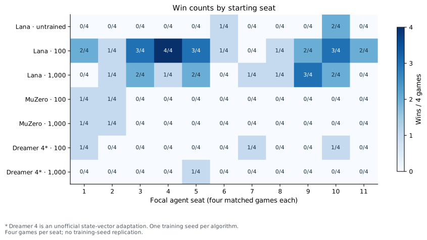
Each common-opponent score comes from 44 matched games against ten frozen untrained Lana agents, balanced across starting seats. The separate mixed tournament puts all six trained checkpoints in each game alongside five untrained agents. It reached the time limit in 19/44 games. Time limits count as no win. Untrained Lana scored 3/44 (6.8%) against common opponents; five untrained tournament entries collectively won 8/44, which is not a single-agent rate.
Bold denotes the numerical row maximum, not statistical significance. Common-opponent 95% Wilson intervals are listed below; they describe game-level uncertainty, not variation across training seeds. No checkpoint was selected using these test games. Lana’s 1,000-game checkpoint scored below its 100-game checkpoint against common opponents.
- Lana · 100: 35.8–64.2%.
- Lana · 1,000: 18.2–44.2%.
- MuZero · 100: 1.3–15.1%.
- MuZero · 1,000: 1.3–15.1%.
- Dreamer 4* · 100: 2.3–18.2%.
- Dreamer 4* · 1,000: 0.4–11.8%.
Lana and MuZero train online; Dreamer uses offline MuZero data. At 100/1,000 games, training update calls are Lana 200/2,000, MuZero 100/1,000, and Dreamer 400/4,000. Calls differ in work and batch size. Lana and MuZero use search; Dreamer uses its policy directly. These are exploratory parameter-matched comparisons, not equal-compute tests or evidence of overall algorithm superiority.
Earlier 11-agent combat study
Controlled combat pilot
Lana & model-based RL baselines
Fixed 100- and 1,000-game training budgets, approximately 3.3 million parameters per model. Each checkpoint faces ten frozen untrained Lana opponents in 44 matched games, balanced across starting seats.
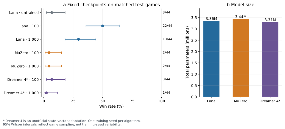
| Model / training games | Wins | Win rate | 95% interval | Time limits |
|---|---|---|---|---|
| Lana · untrained | 3 / 44 | 6.8% | 2.3–18.2% | 2 |
| Lana · 100 | 22 / 44 | 50.0% | 35.8–64.2% | 0 |
| Lana · 1,000 | 13 / 44 | 29.5% | 18.2–44.2% | 0 |
| MuZero · 100 | 2 / 44 | 4.5% | 1.3–15.1% | 12 |
| MuZero · 1,000 | 2 / 44 | 4.5% | 1.3–15.1% | 12 |
| Dreamer 4* · 100 | 3 / 44 | 6.8% | 2.3–18.2% | 0 |
| Dreamer 4* · 1,000 | 1 / 44 | 2.3% | 0.4–11.8% | 2 |
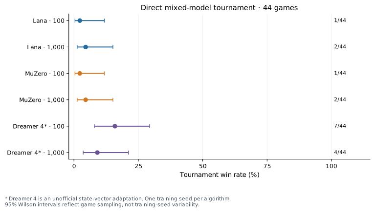
Tournament score table
| Checkpoint | Wins / games | Win rate |
|---|---|---|
| Lana · 100 | 1 / 44 | 2.3% |
| MuZero · 100 | 1 / 44 | 2.3% |
| Dreamer 4* · 100 | 7 / 44 | 15.9% |
| Lana · 1,000 | 2 / 44 | 4.5% |
| MuZero · 1,000 | 2 / 44 | 4.5% |
| Dreamer 4* · 1,000 | 4 / 44 | 9.1% |
Results depend on the opponents: Lana at 100 games led the common-opponent test (22/44 wins). In direct competition, the unofficial Dreamer 4 at 100 games had the most wins among trained entries (7/44), with 19/44 games reaching the time limit. This pilot does not establish an overall best algorithm.
Methods, budgets & limitations
MuZero uses the MuZero-general network with arena-specific history inputs and a small search budget. The unofficial Dreamer 4 adaptation includes shortcut world prediction, behavior cloning and frozen-world imagination training, but replaces the paper’s video architecture with a compact vector model. See the Dreamer 4 paper and MuZero-general source.
Lana and MuZero train online. Dreamer 4 uses offline MuZero self-play data and is fit separately at each data budget. Optimizer steps, observation processing and inference compute differ: Lana and MuZero use MCTS; Dreamer uses its learned policy directly. These are exploratory parameter-matched comparisons, not an equal-compute benchmark or a claim about the original published algorithms.
| Model | Games available | Training update calls | Data |
|---|---|---|---|
| Lana | 100 / 1,000 | 200 / 2,000 | Online self-play |
| MuZero | 100 / 1,000 | 100 / 1,000 | Online self-play |
| Dreamer 4* | 100 / 1,000 | 400 / 4,000 | Offline MuZero games |
Update calls have different batch lengths, losses and internal work; this table does not imply equal optimizer or compute budgets. The common-opponent benchmark is not a direct head-to-head tournament.
All plotted evaluations use the same GPU/backend. A separate CPU audit of the fixed Lana snapshots is preserved; it is not pooled into the plotted rates.
One training seed per algorithm; fixed combat layouts with seeded action sampling and rotated seats. Game-level intervals do not establish reproducibility across training seeds. No checkpoint was selected using these test games. The experiment tests combat winning, not continual learning, retention or general intelligence.
Figure notes · Lana evaluation protocol · Implementation corrections · Compute hardware · Training times & checkpoint hashes
More research